N-Body Simulation: CPU Implementation & Performance Optimization

Where We Left Off

The goal was simple: start with a working single-threaded CPU implementation, and then optimize it before even thinking about GPU code.

This took a while, since I’m juggling this project with college, but it turned into a fascinating deep dive into new optimization strategies and memory caching concepts. What I ended up with was way more interesting than I expected.

The Physics Foundation

Before diving into performance optimizations, let’s talk about the physics being implemented.

Gravitational Acceleration Formula

Newton’s law of universal gravitation gives us the force between two particles. However, since we need to find the acceleration of each particle ( $\vec{a} = \vec{F}/m$ ), it’s more efficient to solve for acceleration directly.

To avoid the simulation blowing up when particles get too close (which would cause a division by zero), a “softening factor” ( $\epsilon^2$ ) is added to the distance. This is a standard and crucial technique in N-body simulations.

The final acceleration formula used is:

$\vec{a}_i = \sum_{j \neq i} G \frac{m_j \vec{r}_{ij}}{(|\vec{r}_{ij}|^2 + \epsilon^2)^{3/2}}$

where $\vec{r}_{ij} = \vec{r}_j - \vec{r}_i$ is the displacement vector from particle i to particle j.

Leapfrog Integration

For time integration, I’m using a highly efficient and stable variant of the leapfrog method called “Kick-Drift-Kick” (KDK). It’s symplectic, meaning it conserves energy well over long periods, which is essential for this kind of simulation.

The KDK algorithm splits the velocity update into two half-steps (“kicks”) separated by a full-step position update (“drift”).

The process for each timestep is:

First Kick (half-step): Velocities are updated by a half-step using the accelerations from the previous frame.
Drift (full-step): Positions are updated by a full-step using these newly modified velocities.
Compute New Accelerations: New accelerations are calculated based on the new particle positions.
Second Kick (half-step): The velocity update is completed with a final half-step using the new accelerations.

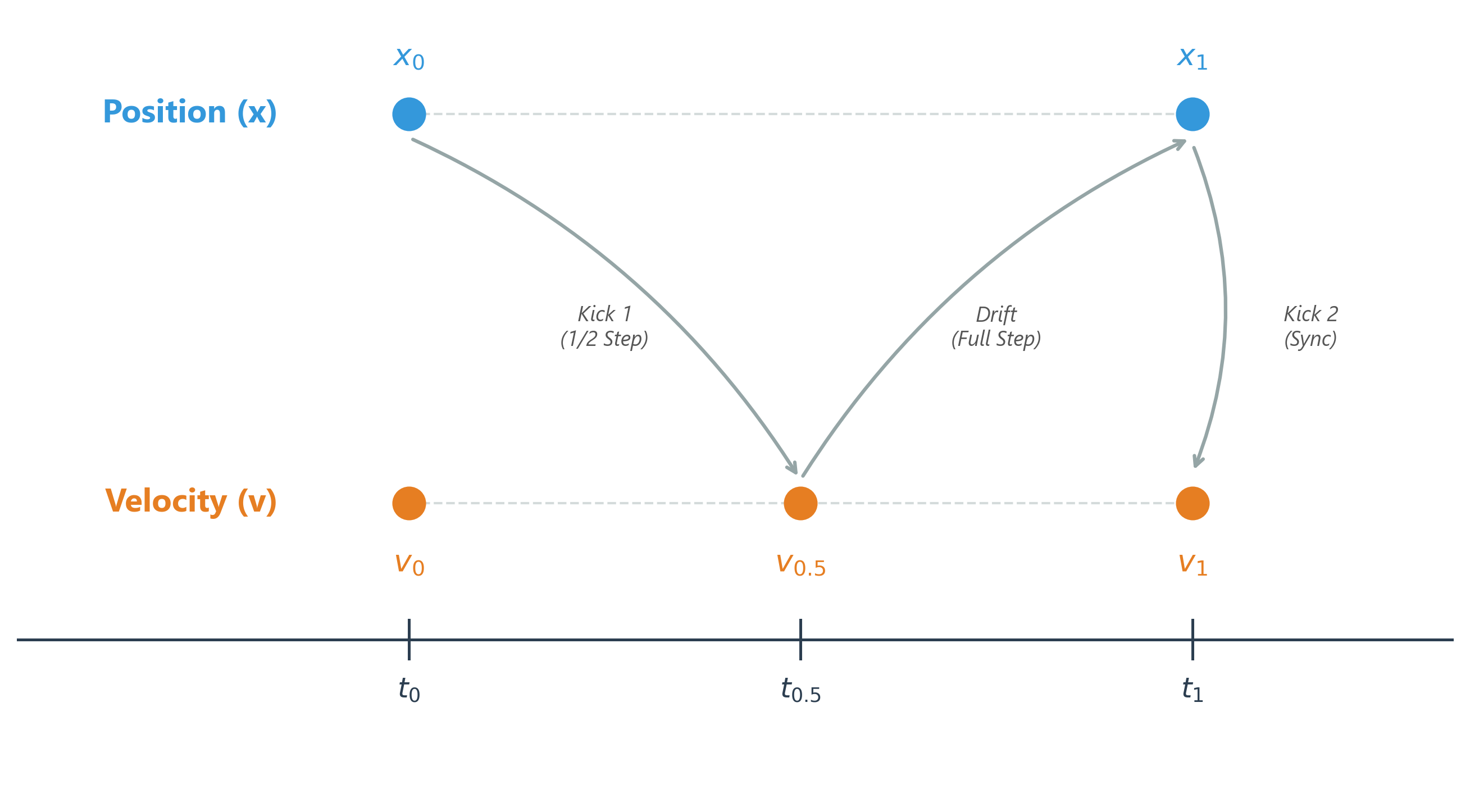
Kick-Drift-Kick Integration Scheme

This “leapfrogging” of position and velocity updates is what gives the method its name and its stability properties.

Setting Up The Foundation

Before I could get to the fun optimization stuff, I first had to knock out all the usual SDL boilerplate to quickly get a window on the screen. It was the standard routine of creating a window, initializing a renderer, and handling events, you know the drill.

Architecture: The Strategy Pattern

I built the physics accelerator system using the classic strategy pattern. There’s an IPhysicsAccelerator interface, and different implementations (CpuAccelerator, CpuAcceleratorPar, and eventually GpuAccelerator) can be swapped at runtime.

This makes benchmarking trivial since the same simulation can be run with different acceleration strategies just by swapping out the accelerator object.

The Memory Layout Story

Here’s where things get really interesting. The performance bottleneck isn’t just parallelization, it’s memory access patterns.

The Problem with Array of Structures

The typical approach would be to have a struct like:

struct Body
{
    float x, y;
    float vx, vy;
    float mass;
};

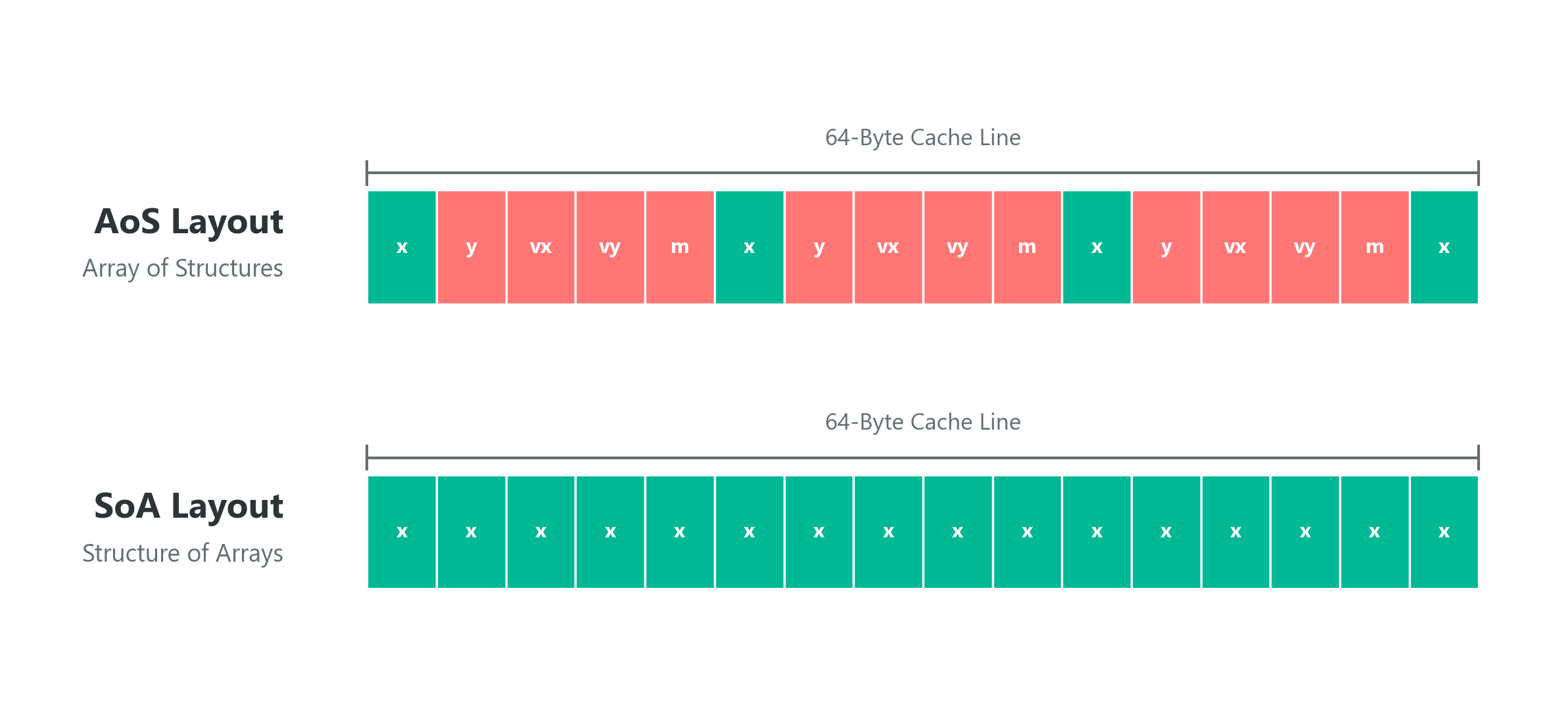
This looks clean in code, but in memory it’s a disaster. When accessing bodies[j].x, an entire cache line gets loaded (64 bytes), but only 4 bytes are used. That’s 93.75% wasted memory bandwidth.

The Solution: Structure of Arrays

Instead of storing particles as an array of structures, what if data is organized as a structure of arrays? That’s exactly what BodiesSoA does:

struct BodiesSoA
{
    using AlignedVector = std::vector<float, AlignedAllocator<float, simd_config::ALIGNMENT>>;

    AlignedVector X;  // Position X
    AlignedVector Y;  // Position Y
    AlignedVector VX; // Velocity X
    AlignedVector VY; // Velocity Y
    AlignedVector M;  // Mass
    
    [[nodiscard]] std::size_t Size() const noexcept
    {
        const std::size_t n = X.size();
        assert(Y.size() == n && VX.size() == n && VY.size() == n && M.size() == n);
        return n;
    }
    
    void Resize(std::size_t n)
    {
        X.resize(n);
        Y.resize(n);
        VX.resize(n);
        VY.resize(n);
        M.resize(n);
    }
};

Now positions are stored contiguously. When accessing positions, 16 consecutive x-coordinates get loaded in one cache line, and 100% of that data gets used.

AoS vs SoA Memory Layout Visualization

Custom Aligned Allocator

To make this work properly, I created a custom aligned allocator that ensures arrays start on 64-byte boundaries (cache line alignment):

template <typename T, std::size_t Alignment> 
class AlignedAllocator
{
    static_assert(Alignment && ((Alignment & (Alignment - 1)) == 0), 
                  "Alignment must be a non-zero power of two");

public:
    using value_type = T;

    [[nodiscard]] T* allocate(std::size_t n)
    {
        if (n == 0) [[unlikely]]
            return nullptr;
        if (n > (std::numeric_limits<std::size_t>::max() / sizeof(T))) [[unlikely]]
            throw std::bad_array_new_length();

        const std::size_t bytes = n * sizeof(T);

#ifdef _MSC_VER
        void* p = _aligned_malloc(bytes, Alignment);
        if (!p)
            throw std::bad_alloc();
        return static_cast<T*>(p);
#else
        // Platform-specific allocation code
#endif
    }

    void deallocate(T* p, std::size_t) noexcept
    {
        if (!p)
            return;
#ifdef _MSC_VER
        _aligned_free(p);
#else
        std::free(p);
#endif
    }
};

This guarantees proper cache line alignment for maximum memory bandwidth utilization.

The Parallel Implementation

For parallelization, I chose Intel’s Threading Building Blocks (TBB) over alternatives like OpenMP. TBB has task-based parallelism with automatic load balancing and a work-stealing scheduler that handles uneven workloads beautifully. TBB automatically redistributes work from busy threads to idle ones, maintaining load balance without manual intervention.

Here’s the core update loop in CpuAcceleratorPar:

void CpuAcceleratorPar::Update(BodiesSoA& bodies, float dt)
{
    const std::size_t n = bodies.Size();
    if (n == 0) [[unlikely]]
        return;

    if (m_accX.size() != n) [[unlikely]]
    {
        m_accX.resize(n, 0.0f);
        m_accY.resize(n, 0.0f);
    }

    constexpr float g = 6.67430e-11f;
    constexpr float softening2 = 1e-9f;
    const float dtHalf = 0.5f * dt;
    constexpr std::size_t kGrainSize = 1;

    float* RESTRICT pVx = bodies.VX.data();
    float* RESTRICT pVy = bodies.VY.data();
    float* RESTRICT pX = bodies.X.data();
    float* RESTRICT pY = bodies.Y.data();
    float* RESTRICT pAccX = m_accX.data();
    float* RESTRICT pAccY = m_accY.data();

    oneapi::tbb::parallel_for(oneapi::tbb::blocked_range<std::size_t>(0, n, kGrainSize),
                              [&](const oneapi::tbb::blocked_range<std::size_t>& r) {
                                  KickDriftRange(r.begin(), r.end(), pVx, pVy, pX, pY, 
                                                pAccX, pAccY, dt, dtHalf);
                              });
    
    // Compute accelerations...
    // Final kick...
}

The Vectorization Tricks

Here’s where it gets kinda tricky. When I first ran this code, I ran into some classic compiler quirks. MSVC’s /Qvec-report:2 flag showed that some loops weren’t getting vectorized. This flag tells the compiler to report which loops were vectorized and which weren’t, along with the reasons why.

Compiler Hints Header

To give the compiler more confidence, I defined a few platform-specific macros that provide the necessary optimization hints.

#ifdef _MSC_VER
#define RESTRICT __restrict
#define FORCE_INLINE __forceinline
#define PRAGMA_IVDEP __pragma(loop(ivdep))
#elifdef __clang__
#define RESTRICT __restrict__
#define FORCE_INLINE inline __attribute__((always_inline))
#define PRAGMA_IVDEP _Pragma("clang loop vectorize(assume_safety)")
#elifdef __GNUC__
#define RESTRICT __restrict__
#define FORCE_INLINE inline __attribute__((always_inline))
#define PRAGMA_IVDEP _Pragma("GCC ivdep")
#else
#define RESTRICT
#define FORCE_INLINE inline
#define PRAGMA_IVDEP
#endif

Let’s break down what each of these does:

RESTRICT: This keyword tells the compiler that pointers don’t alias each other. When marking a pointer as RESTRICT, it’s promising the compiler that any data written through that pointer isn’t read by any other restricted pointer. This allows the compiler to reorder and optimize operations without worrying about hidden dependencies.

FORCE_INLINE: Forces the compiler to inline the function, eliminating function call overhead. For tiny hot-path functions like the ones here, inlining is crucial.

PRAGMA_IVDEP: This is the vectorization magic. ivdep stands for “ignore vector dependencies”. It tells the compiler to ignore conservatively assumed data dependencies that would prevent vectorization. Basically saying “trust me, there are no loop-carried dependencies here, go wild with SIMD.”

The Kick-Drift Function

Here’s how these hints are applied in practice:

static FORCE_INLINE void KickDriftRange(std::size_t begin, std::size_t end, 
                                       float* RESTRICT pVx, float* RESTRICT pVy,
                                       float* RESTRICT pX, float* RESTRICT pY, 
                                       const float* RESTRICT pAccX,
                                       const float* RESTRICT pAccY, 
                                       float dt, float dtHalf) noexcept
{
    float* RESTRICT vx = std::assume_aligned<simd_config::ALIGNMENT>(pVx);
    float* RESTRICT vy = std::assume_aligned<simd_config::ALIGNMENT>(pVy);
    float* RESTRICT x = std::assume_aligned<simd_config::ALIGNMENT>(pX);
    float* RESTRICT y = std::assume_aligned<simd_config::ALIGNMENT>(pY);
    const float* RESTRICT accX = std::assume_aligned<simd_config::ALIGNMENT>(pAccX);
    const float* RESTRICT accY = std::assume_aligned<simd_config::ALIGNMENT>(pAccY);

    PRAGMA_IVDEP
    for (std::size_t i = begin; i < end; ++i)
    {
        vx[i] += accX[i] * dtHalf;
        vy[i] += accY[i] * dtHalf;
        x[i] += vx[i] * dt;
        y[i] += vy[i] * dt;
    }
}

RESTRICT pointers to tell the compiler about non-aliasing
std::assume_aligned to guarantee 64-byte alignment (important for AVX-512)
PRAGMA_IVDEP right before the loop to enable vectorization

After adding these hints, /Qvec-report:2 confirmed all loops were successfully vectorized. Beautiful.

The Acceleration Computation with Tiling

The acceleration computation uses a tiling optimization for cache efficiency:

static FORCE_INLINE void ComputeAccelerationTile(const float* RESTRICT xConst, 
                                                 const float* RESTRICT yConst,
                                                 const float* RESTRICT mConst, 
                                                 float piX, float piY, 
                                                 std::size_t jBase,
                                                 std::size_t jEnd, 
                                                 float& ax, float& ay, 
                                                 float softening2) noexcept
{
    const float* RESTRICT x = std::assume_aligned<simd_config::ALIGNMENT>(xConst);
    const float* RESTRICT y = std::assume_aligned<simd_config::ALIGNMENT>(yConst);
    const float* RESTRICT m = std::assume_aligned<simd_config::ALIGNMENT>(mConst);

    float axLocal = 0.0f;
    float ayLocal = 0.0f;

    PRAGMA_IVDEP
    for (std::size_t j = jBase; j < jEnd; ++j)
    {
        const float dx = x[j] - piX;
        const float dy = y[j] - piY;
        const float dist2 = (dx * dx) + (dy * dy) + softening2;
        const float inv = 1.0f / std::sqrtf(dist2);
        const float inv3 = inv * inv * inv;
        const float s = m[j] * inv3;
        axLocal += dx * s;
        ayLocal += dy * s;
    }

    ax += axLocal;
    ay += ayLocal;
}

After testing different tile sizes (256, 512, 1024), 512 ended up being the sweet spot for my specific hardware. The goal is to keep the working set in L2 cache to minimize memory latency.

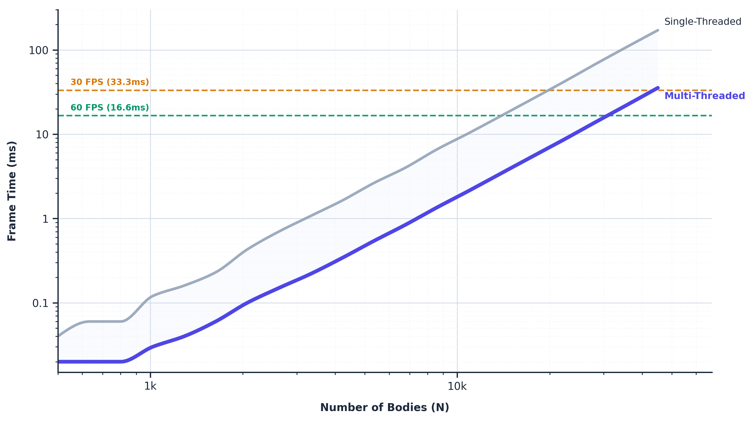
Putting all these optimizations together yields substantial performance gains. The benchmark below compares the single-threaded implementation against the optimized TBB parallel version, showcasing how the parallel approach manages the $O(N^2)$ complexity much better as the particle count grows.

N-Body Simulation Performance Benchmark

What’s Next

Now that the CPU code is optimized, the next phase of this project is all about the GPU. The plan is to build out the CUDA implementation and then put it head-to-head with the CPU version in a series of performance benchmarks.